bm424

Implementing Functional Graph Algorithms in Python (Part 3: Algorithms)

I’ll show you how to implement topological sorting and Dijkstra’s algorithm for shortest paths using functional methods. We’ll use new Python features like `match` statements to get very close to the declarative Haskell description of these algorithms.

Welcome back to this series on functional programming in Python! We’ve been looking at how to implement inductive graphs ( Erwig 2001) in Python. In the first part, we looked at how to implement the necessary data types, and in the second part we implemented some basic functions.

In this section, I’ll show you how to implement topological sorting and Dijkstra’s algorithm for shortest paths using the methods described in the paper. We’ll use new Python features like match statements to get very close to the declarative Haskell description of these algorithms.

Topological Sorting

A topological sort of a graph is a list of its nodes which are followed in an order where “earlier” nodes come before "later" nodes (for a more precise definition see the linked Wikipedia article). Strictly speaking, this is only possible if the graph is acyclic — this means there are no loops. It’s useful for resolving the “order” that processes should be evaluated in if, for example, your graph represents data flow. Topological sorts are not unique.

Depth-First Forest

The paper describes an inductive graph algorithm for the topological sort which relies on a "depth-first forest" which can be derived from the graph. What is this?
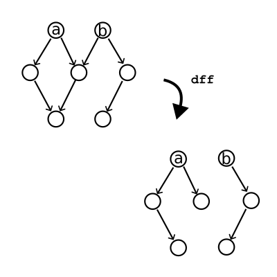
A single graph with seven nodes, the first two labeled 'a' and 'b', with directed edges joining some of the other nodes. An arrow labeled 'dff' shows the transformation to the depth first forest. The forest shows the same seven nodes, but 'a' and 'b' now represent the roots of two separate subtrees.

We can decompose the graph into a number of “trees”. Trees are like graphs but nodes only ever have one predecessor. Starting at any node, we can get a single tree by removing it and following successors until we run out of nodes. To get the forest, we just need to start searching from all nodes. The algorithm described in Haskell notation looks like this:

df :: [Node] -> Graph a b -> ([Tree Node], Graph a b)
df [] g = ([], g)
df (v:vs) (c &v g) = (Br v f:f', g₂) where (f, g₁) = df (suc c) g; (f', g₂) = df vs g₁
df (v:vs) g = df vs g

Implementation

Phew! That’s a confusing definition. Let’s break it down in Python. Firstly, the function says that given a queue of nodes [Node] and a graph Graph a b, df returns a tuple (a Haskell-style tuple with a fixed length). The first element of the tuple is a queue of trees of nodes, and the second is a graph. Since we’re using methods to implement these functions in Python, it’s almost the same:

class Graph(abc.ABC, typing.Generic[A, B]):
    ...

    def _dff(self, nodes: tuple[Node, ...]) -> tuple[tuple[Tree[Node], ...], "Graph[A, B]"]:
        ...

The next line, df [] g = ([], g), says that if there are no nodes, we just return an empty tuple and the graph itself:

class Graph(abc.ABC, typing.Generic[A, B]):
    ...

    def _dff(self, nodes: tuple[Node, ...]) -> tuple[tuple[Tree[Node], ...], "Graph[A, B]"]:
        if not nodes:
            return (), self
        ...

The line after this, df (v:vs) (c &v g) = (Br v f:f', g₂) where (f, g₁) = df (suc c) g; (f', g₂) = df vs g₁, says: if we can find the first node, v, in the graph, then calculate the forest for all of the successors of that node in the graph without that node. Then, carry on calculating trees with whatever nodes vs we haven’t yet looked at. We then construct a tree with the node at the head of the forest of successors, then return it alongside all the other trees we’ve found.

class Graph(abc.ABC, typing.Generic[A, B]):
    ...

    def _dff(self, nodes: tuple[Node, ...]) -> tuple[tuple[Tree[Node], ...], "Graph[A, B]"]:
        ...
        head, *tail = nodes  # (v:vs)
        match self.pop(head):  # (c &v g)
            case c, g:
                f, g1 = g._dff(c.suc)  # (f, g1) = df (suc c) g
                f_, g2 = g1._dff(tuple(tail))  # (f', g2) = df vs g1
                return (Tree(head, f), *f_), g2  # (Br v f:f', g2)

Why have I used match-case here? Well, what happens if we can’t find the node v in the graph? We just carry on with the other nodes, as in the final line of the algorithm df (v:vs) g = df vs g:

class Graph(abc.ABC, typing.Generic[A, B]):
    ...

    def _dff(self, nodes: tuple[Node, ...]) -> tuple[tuple[Tree[Node], ...], "Graph[A, B]"]:
        ...
        head, *tail = nodes  # (v:vs)
        match self.pop(head):  # (c &v g)
            case c, g:
                ...
            case None:
                return self._dff(tuple(tail))  # df vs g

So the match statement allows a nice clean syntax demonstrating both cases.

Finally, we can wrap the whole thing in a public dff method which just passes all of the graph’s nodes into the function, so that we get back a forest that spans the whole graph:

class Graph(abc.ABC, typing.Generic[A, B]):
    ...

    def _dff(self, nodes: tuple[Node, ...]) -> tuple[tuple[Tree[Node], ...], "Graph[A, B]"]
        ...

    def dff(self):
        return self._dff(self.nodes())[0]

The topological sort of the graph is derived from the depth-first spanning forest. We can walk through each tree from the bottom up (using a function called postOrder). The reverse of this sequence is a topological sort!

class Graph(abc.ABC, typing.Generic[A, B]):
    ...

    def _dff(self, nodes: tuple[Node, ...]) -> tuple[tuple[Tree[Node], ...], "Graph[A, B]"]
        ...

    def dff(self) -> tuple[Tree[Node], ...]:
        return self._dff(self.nodes())[0]

    def topsort(self) -> tuple[Node, ...]:
        return tuple(reversed(concat_map(Tree.post_order, self.dff())))

Isn't that sweet?

Dijkstra's Shortest Path Algorithm

Finally, let’s implement the inductive graph version of Dijkstra’s shortest path algorithm. There’s a bit of underlying machinery here involving what the paper calls LRTrees and LPaths which I won’t get in to here, but feel free to take a look at the code. The important thing for the implementation is that LPaths are labeled lists of nodes which can be compared using < — i.e. one is “shorter” than another. This means they can be used in a heap.

Definition

dijkstra :: Real b => Heap (LPath b) -> Graph a b -> LRTree b

This says that for a graph with node edges labeled with a real number, and a heap (a data structure where we can efficiently get the smallest value) of paths, dijkstra will return a LRTree (a queue of labeled paths) representing the shortest paths between a given node and all other reachable nodes.

dijkstra h g | isEmptyHeap h || isEmpty g = []

Simple enough: there are no short paths in an empty graph. For non-empty graphs, the heap should never be empty, because we always have a zero-length path from a node to itself.

dijkstra (p@((v,d):_)≺h) (c &v g) = p:dijkstra (mergeAll h:expand d p c)) g

😱 What is this nightmare? In words, it says: if the first node v in the smallest path p in the heap can be found in the graph, return that path and keep searching with v removed and a heap with that path removed and a set of new paths starting at all the successors. What this means is that when a new, shorter path to a given node is found it replaces the existing one.

Finally, if the shortest path’s first node v is not in the graph, we can just carry on with trying to find shorter paths than the ones we’ve got:

dijkstra (_≺h) g = dijkstra h g

Implementation

Like the topological sort, this algorithm maps very nicely to Python. I’ve included the _expand method for completeness:

class Graph(abc.ABC, typing.Generic[A, B]):
    ...

    @staticmethod
    def _expand(
            item: float, lpath: "LPath[float]", context: Context[A, float]
    ) -> tuple[ImmutableHeap["LPath[float]"], ...]:
        return tuple(
            ImmutableHeap.unit(LPath((LNode(node, item + label), *lpath)))
            for label, node in context.successors
        )

    def _dijkstra(self, heap: ImmutableHeap["LPath[float]"]) -> "LRTree[float]":
        if not heap or self.is_empty:  # isEmptyHeap h || isEmpty g
            return LRTree()
        p, h = heap.pop()  # p < h
        (v, d), *_ = p  # p@((v, d): _)
        match self.pop(v):  # c &v g
            case (c, g):
                return LRTree(
                    (p, *g._dijkstra(ImmutableHeap.merge(heap, *self._expand(d, p, c))))
                )  # p:dijkstra (mergeAll (h:expand d p c) g
            case None:
                return self._dijkstra(h)  # dijkstra h g

With a list of shortest paths, we now just need some wrapper functions to complete the implementation:

class Graph(abc.ABC, typing.Generic[A, B]):
    ...

    def _spt(self, node: Node) -> "LRTree[float]":
        heap = ImmutableHeap.unit(LPath((LNode(node, 0.0),)))
        return self._dijkstra(heap)

    def sp(self, s: Node, t: Node) -> tuple[Node, ...] | None:
        return self._spt(s).get_path(t)

Note that there is a typo in the linked version of the paper which incorrectly defines spt, i.e. the shortest paths from t, as

spt v = spt (unitheap [(v, 0)])

where it should read

spt v = dijkstra (unitheap [(v, 0)])

Validation

Let’s check it works! Wikipedia has an article on Dijkstra’s algorithm where it shows a simple small graph labeled 1–6.
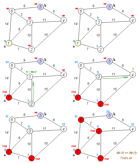
An animation demonstrating Dijkstra's algorithm implemented the 'normal' way, showing an undirected, labeled graph with six nodes. Starting at the node labeled '1', the animation shows how each node is visited in turn and tagged with a value representing the shortest path to that node, until the shortest path to the destination is tagged. The final shortest path is 1, 3, 6, 5, with a total length of 20

The shortest graph from Node 1 to Node 5 goes through 3 and 6. Given everything we’ve implemented so far, we can now construct this graph with all the edges and test our algorithm:

>>> graph = (
...     Context(Adj(), Node(1), 1, Adj(((7, Node(2)), (9, Node(3)), (14, Node(6)))))
...     & Context(Adj(), Node(2), 2, Adj(((10, Node(3)), (15, Node(4)))))
...     & Context(Adj(), Node(3), 3, Adj(((11, Node(4)), (2, Node(6)))))
...     & Context(Adj(), Node(4), 4, Adj(((6, Node(5)),)))
...     & Context(Adj(), Node(5), 5, Adj(((9, Node(6)),)))
...     & Context(Adj(), Node(6), 6, Adj())
...     & EmptyGraph()
... ).undir()
>>> graph.sp(Node(1), Node(5))
(1, 3, 6, 5)

That puts a smile on my face.

Conclusion

We’ve seen how to implement some functional algorithms for graphs in Python, and how closely we can approach the Haskell descriptions using Python syntax like destructuring and match statements. In the next and final part I’m going to give my overall thoughts about this exercise, and draw some conclusions about functional programming in Python. See you there!

References

  1. Erwig, Martin. “Inductive graphs and functional graph algorithms.” Journal of Functional Programming 11.5 (2001): 467–492.
  2. Wikipedia contributors. "Dijkstra's algorithm." Wikipedia, The Free Encyclopedia https://en.wikipedia.org/w/index.php?title=Dijkstra%27s_algorithm&oldid=1357396357.
Implementing Functional Graph Algorithms in Python (Part 2: Functions)

Implementing the necessary abstract methods and some basic algorithms.

Hello! Welcome to the second part of this series on functional programming in Python. If you haven’t read the first part yet, check it out here.

In this series, we’re implementing “inductive graphs” as described in this paper ( Erwig 2001). In the first part, we defined the basic data structures, and we’ll now move on to implementing the necessary abstract methods and some basic algorithms. As a reminder, you can find all of the code for these articles at the inductive-graph-algorithms repository over on GitHub.

Abstract Methods

Take a look at Table 1 in the paper. It explains that for inductive graph algorithms, we need three basic features for the graph:

  1. A test for emptiness.
  2. The ability to extract an arbitrary context from the graph.
  3. The ability to extract a specific context from the graph.

How we choose to implement these features is up to us. I’ve chosen to implement the test for emptiness as a property of the graph, and the context extraction as a method .pop(node: Optional[Node]) on the graph:

class Graph(abc.ABC, typing.Generic[A, B]):
    ...

    @property
    @abc.abstractmethod
    def is_empty(self) -> bool:
        """True if the graph is empty (contains no nodes), False otherwise."""

    @abc.abstractmethod
    def pop(self, node: Node | None = None) -> tuple[Context[A, B], "Graph[A, B]"] | None:
        """Extracts a given `node` from the graph.

        Returns the node's context, and the remaining graph. If `node` is None, any
        node may be extracted. If `node` is not in the graph, returns None.
        """

Now let’s implement these for our subtypes! For the empty graph, it’s easy enough:

class EmptyGraph(Graph[A, B]):
    ...

    @property
    def is_empty(self) -> bool:
        return True

    def pop(self, node: Node | None = None) -> tuple[Context[A, B], "Graph[A, B]"] | None:
        return None

The empty graph is, obviously, empty, and we can never extract any context from it.

The inductive graph implementation is more complicated:

class InductiveGraph(Graph[A, B]):
    ...

    @property
    def is_empty(self) -> bool:
        return False

    def pop(self, node: Node | None = None) -> tuple[Context[A, B], "Graph[A, B]"] | None:
        if node is None or node == self.head.node:
            return self.head, self.tail
        node_context, graph_context = self.head.pop(node)
        if match := self.tail.pop(node):
            sub_node_context, subgraph = match
            return node_context | sub_node_context, graph_context & subgraph
        return None

Let’s dig into pop here.

First, if node is None, it means we can return any arbitrary context alongside the remaining graph. The way we’ve implemented InductiveGraph makes this very easy — we simply return the head, which is a context, and the tail, which by construction never refers to any node mentioned in the head. We can do exactly the same if the specific node requested happens to be the head node.

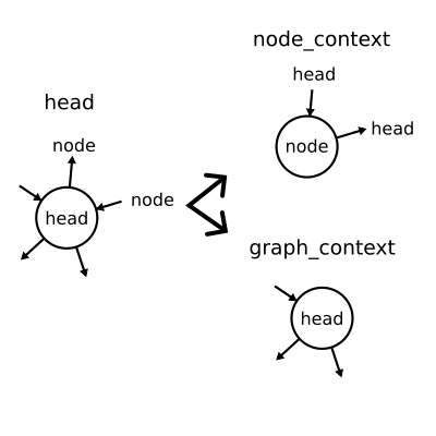
If neither of the two conditions above is satisfied, it’s time for some recursion! First, we take the head context and split it into two parts. The first part contains any references to node, inverted so that node is the node of the context — this is node_context. The second part contains any references that are not to node.

An illustration of how the "head" node of a graph is decomposed into two contexts. One context, called "node_context", centres on "node", and contains only references between "node" and "head". The other context, called the "graph_context", centres on "head", and contains only any other references to "head".

Then, we try to pop node from tail, meaning that we start again with pop! Eventually, we must either reach node, or find that node is not in the graph. Either way, the recursion terminates at some point.

What happens if we reach node? pop returns a tuple of node_context | sub_node_context and graph_context & subgraph. The first part of this joins all of the node_contexts together into a single context - the one we want extracted! Every reference to node in the graph is encapsulated in a new context with node at the center. The second part re-constructs a graph from all of the contexts which don't contain node - the remainder.

That's a lot of behaviour wrapped up in one little function, so let's go over it slowly once more.

  1. If the head is the context of the node we need, return it and the remaining graph.
  2. Otherwise, break the head into parts. One part contains any references to the node we need, the other part contains no references to the node we need.
  3. Repeat the above process with the tail.
  4. Once we have the context of the node we need, join all the contexts that do reference the node into our extracted context, and construct a graph from the contexts that do not reference the node.

Phew 😅 With that tricky part out the way, we can get on to some sweet implementations!

Basic Functions

Back in Part 1, I said that we could define functions on inductive graphs analogous to reduce and map for lists. Let's do that now!

ufold()

In the paper, reduce for graphs is called ufold. fold is an often-used synonym for reduce in functional programming, and ufold means the fold on graphs is "unordered," because the nodes are, in general, traversed in arbitrary order.

The paper describes the ufold function in the following way:

ufold :: (Context a b -> c -> c) -> c -> Graph a b -> c
ufold f u Empty = u
ufold f u (c & g) = f c (ufold f u g)

This means: take a graph, a starting value of type c, and a function which takes something of type c and a Context to produce a result c. ufold will then produce a result of type c. Yes, it's a higher-order function which takes another function as a parameter! ufold over an empty graph is just the starting value, but for anything else we extract an arbitrary context, then apply the function over that context and the result of ufold on the remainder. More recursion!

Thankfully, this is actually pretty concise in Python:

class Graph(abc.ABC, typing.Generic[A, B]):
    ...

    def ufold(self, fn: typing.Callable[[Context[A, B], C], C], u: C) -> C:
        """Un-ordered fold."""
        if self.is_empty:
            return u
        head, graph = self.pop()  # c & g
        return fn(head, graph.ufold(fn, u))  # f c (ufold f u g)

nodes()

How do we use .ufold()? Well, let's say we want to get the nodes of the graph. In Haskell syntax, the function looks like this:

nodes :: Graph a b -> [Node]
nodes = ufold (\(p, v, l, s) -> (v:)) []

In simple words, this says that the nodes of the graph are just appended one by one to an initially-empty list. In Python, it looks like this:

class Graph(abc.ABC, typing.Generic[A, B]):
    ...

    def nodes(self) -> tuple[Node, ...]:
        """The nodes of the graph."""
        # ufold (\(p, v, l, s) -> (v:)) []
        return self.ufold(lambda context, result: (context.node, *result), ())

That's pretty concise, and again it mirrors the Haskell definition pretty closely.

gmap()

gmap is the graph's equivalent of map and we can use ufold to implement it!

gmap :: (Context a b -> Context c d) -> Graph a b -> Graph c d
gmap f = ufold (\c -> (f c &)) Empty

In other words, gmap is a function that takes a graph and a function that converts a context into another context, and produces another graph. We can implement it by applying the function to each context, and constructing a graph from the result. In Python:

class Graph(abc.ABC, typing.Generic[A, B]):
    ...

    def gmap(
            self, fn: typing.Callable[[Context[A, B]], Context[C, D]]
    ) -> "Graph[C, D]":
        """Convert the graph into another graph via `fn` over its contexts."""
        # ufold (\c -> f c &) Empty
        return self.ufold(
            lambda context, result: fn(context) & result, EmptyGraph[C, D]()
        )

Conclusion

The inductive graph definition requires just three features: a test for emptiness, the removal of an arbitrary node's context, and the removal of a specific node's context. With those in place, we can create some very succinct functions to form the basis of our functional graphs: ufold, and gmap.

In the next part, we'll implement some more complex algorithms including Dijkstra's algorithm and topological sorting.

References

  1. Erwig, Martin. "Inductive graphs and functional graph algorithms." Journal of Functional Programming 11.5 (2001): 467–492.

Implementing Functional Graph Algorithms in Python (Part 1: Data Types)

I'd like to show you a challenging functional programming problem, and demonstrate that Python has a great syntax for writing elegant, concise functional code.

If you've ever read articles about functional programming in Python, you probably already know about map, filter, and reduce, which are useful functions for functional programming using lists. However, if you're like me, you may have sometimes felt that articles like that are a bit shallow, and don't really teach you anything about how to use Python as a functional programming language in general. I'd like to show you a more challenging functional programming problem, and demonstrate that Python has a great syntax for writing elegant, concise functional code.

This will be a four-part series. In this part, I'll be describing the problem of functional graph algorithms, and setting up basic data structures. In Part 2, I'll implement the basic functions we'll need to write more expressive algorithms, which we'll cover in Part 3. Finally, I'll give you my final thoughts on this exercise (a "retro", if you like) in Part 4.

You can find all of the code for these articles at the inductive-graph-algorithms repository over on GitHub.

The Problem

Many programmers will have had to do some work with data structures like trees, such as JSON data or web documents, or graphs, such as are used in data processing frameworks like Airflow. A few months ago, I was working on designing a system with a graph-like structure. I'm a big fan of functional programming, so I started wondering: how does a functional program implement algorithms like topological sorting?

In the world of imperative programming, topological sorting is not very difficult — Kahn's algorithm and a depth-first search algorithms are both described on the Wikipedia page linked above. However, both rely on stateful mutations of the graph's nodes, because they need us to keep track of visited nodes via a label. Stateful changes should not be part of our functional implementation.

The Solution

After a little bit of googling, I came across this paper (Erwig 2001), which describes the principle of "inductive" graphs, and forms the basis of Haskell's functional graph library fgl. I'll try to quickly explain inductive graphs by analogy to a list, but for a more detailed explanation see this StackExchange answer and its linked blog post — they're both excellent.

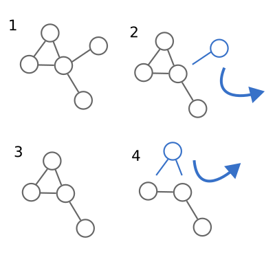
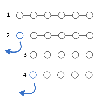
When we take a sequence like a list or a tuple, and remove an item, we produce a pair: the item, and a new list or tuple with all the existing items except for the one we just removed. We can then repeat the operation on the new list. Functions like map, filter, and reduce can be concisely defined because of this repetition.

A diagram with four parts, representing generalised functional operations on sequences. In part 1, a series of 5 circles are joined together with lines, representing a list. In part 2, the first circle is separated and highlighted, representing its removal and usage in some functional operation. Part 3 shows the 4 remaining circles, and part 4 shows the removal of the first circle as in part 2.

Basic operation for functions over lists: 1) Start with a list of any length. 2) Remove the first item and perform some operation. 3) You now have a smaller list. 4) Repeat from step 2.

An inductive graph has a similar property. Instead of removing a single item, we remove a node and all of its connected edges, returning a graph without any reference to the node we just removed. We can then repeat the operation on the new graph. This means we can define functions analogous to map, filter, and reduce for an inductive graph, and go further, implementing depth-first walks, shortest-path algorithms, and, indeed, topological sorts.

A diagram with four parts, representing generalised functional operations on graphs. In part 1, a series of 5 circles are joined together with lines, representing a graph. In part 2, an arbitrary circle is separated and highlighted, representing its removal and usage in some functional operation. Part 3 shows the 4 remaining circles, and part 4 shows the removal of another arbitrary circle as in part 2.

Basic operation for inductive functions over graphs: 1) Start with any graph. 2) Remove a node and all of its edges and perform some operation. 3) You now have a smaller graph. 4) Repeat from step 2.

Implementation

Notes

The paper describes its data structures and functions in Haskell syntax, so we need to work out how to convert this into Python. I've generally adopted the following approach:

  1. Types and data types are implemented as classes, and where the types need to be destructured I've implemented __iter__ so that we can use Python's destructuring (for example x, *y = […]) to closely match the definition.
  2. I've implemented most of the functions as methods on the classes, rather than external functions, because it keeps the code organised and "more Pythonic".
  3. "Queues" are ordered sequences — I've used tuples rather than lists to prevent accidental mutation. In some algorithms, the order doesn't matter and for these cases I've used the builtin frozenset, rather than plain sets, again to avoid accidental mutation.
  4. Later in the paper, a "heap" is used for shortest-path algorithms. Python has built-in efficient heap algorithms in the heapq package, but these rely on mutating lists in-place. I implemented a wrapper class which helps ensure immutability.

Node

The very first type described in the paper is the type

type Node = Int

That's right, nodes are integers. Actually, we can think of this as being like the index of an item in the list — the node type is the "index" of the node in the graph. In Python:

class Node(int):
    """A node.

    For convenience, nodes are represented by integers.
    """

Simple!

"Adj"

type Adj b = [(b, Node)]

This is a bit more abstract. It means that Adj is a sequence of tuples. Each tuple represents an edge in the graph, and b represents the edge's label, which can be anything, so we leave it generic. Note that edges are directed: Adj may describe a connection to or from a given node, but by itself it doesn't care which.

class Adj(collections.abc.Sequence[tuple[B, Node]]):
    """Adjacency relationships."""

    labeled_nodes: tuple[tuple[B, Node], ...]

    def __init__(self, labeled_nodes: tuple[tuple[B, Node], ...] = ()):
        self.labeled_nodes = labeled_nodes

    def __repr__(self):
        return f"Adj({self.labeled_nodes!r})"

    def __len__(self):
        return len(self.labeled_nodes)

    def __getitem__(self, item):
        return self.labeled_nodes[item]

    def __eq__(self, other):
        return self.labeled_nodes == other.labeled_nodes

    def __add__(self, other):
        return Adj(self.labeled_nodes + other.labeled_nodes)

I've made this class inherit from the Sequence class, which means if we implement __len__ and __getitem__ we get iteration for free. I've also specified __eq__ and __add__ so that the class behaves like a tuple.

Context
type Context a b = (Adj b, Node, a, Adj b)

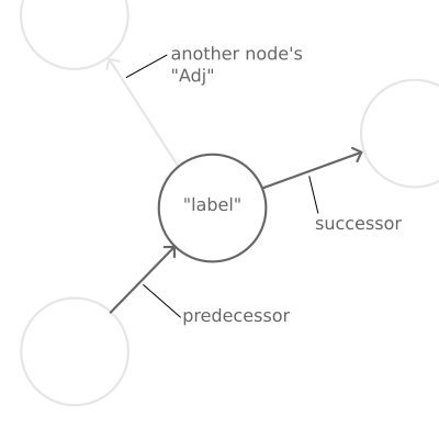
More abstract again! This says that a "context" comprises four parts: an adjacency relationship, a node, the label of that node (a), and another adjacency relationship. The first Adj represents edges directed towards Node, called "predecessors", and the second Adj represents edges directed away from Node, called "successors". It's important to note that, for inductive graphs, this doesn't have to be all of the connected nodes, because other Contexts may define additional Adj relationships.

There are two generic types here: a is the type of the node's label, and b is the type of the edge's label.

A diagram showing the "context" of a node in an inductive graph. There are four circles, of which one is central and highlighted. It has a highlighted arrow, labelled "predecessor", directed towards it from one of the other circles. Another highlighted arrow, labelled "successor" is directed out of it toward one of the other circles. Another arrow, not highlighted, points towards the last circle, and is labelled "Another node's ‘Adj'".

Anatomy of a "Context": predecessor edges pointing to this node, successor edges pointing away from this node, and a label of arbitrary type on the node itself. Note that a "Context" doesn't necessarily refer to all of the edges connecting into a node, because these might be parts of other "Context"s.

class Context(typing.Generic[A, B]):
    """A context.

    A node's context describes (some of) its surroundings, including its label, its 
    adjacent predecessors and its adjacent successors.
    """

    predecessors: Adj[B]
    node: Node
    label: A
    successors: Adj[B]

    def __init__(
            self,
            predecessors: Adj[B],
            node: Node,
            label: A,
            successors: Adj[B],
    ):
        self.predecessors = predecessors
        self.node = node
        self.label = label
        self.successors = successors

    def __repr__(self):
        return f"Context({self.predecessors!r}, {self.node!r}, {self.label!r}, {self.successors!r})"

    def __eq__(self, other):
        return (
                self.predecessors == other.predecessors
                and self.node == other.node
                and self.label == other.label
                and self.successors == other.successors
        )

Graph

Finally, we can describe a graph itself:

data Graph a b = Empty | Context a b & Graph a b

This says that a graph is either an empty graph OR a context attached (using the operator &) to a graph.

Python doesn't have variant types like this, but we can use inheritance instead. We'll define an abstract Graph class that will have two subclasses: EmptyGraph and InductiveGraph.

class Graph(abc.ABC, typing.Generic[A, B]):
    """An abstract graph""" 

The InductiveGraph will contain a "head", which is the Context a b, and a "tail", which is another graph.

class EmptyGraph(Graph[A, B]):
    """An empty graph, containing no nodes or edges."""

    def __repr__(self):
        return "EmptyGraph"
class InductiveGraph(Graph[A, B]):
    """An inductive graph.

    The `head` of the graph is a context that can only refer to nodes in the `tail`,
    which is also a graph.
    """

    head: Context[A, B]
    tail: Graph[A, B]

    def __init__(self, head: Context[A, B], tail: Graph[A, B]):
        self.head = head
        self.tail = tail

    def __repr__(self):
        return f"{self.head!r} & {self.tail!r}"

Construction

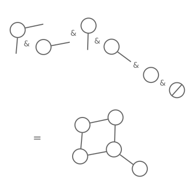
As well as the data itself, we can implement the constructor operator & using Python! In the paper, we imagine building up graphs right-to-left, starting with the empty graph, and adding on context until we reach the whole graph:

Context(...) & Context(...) & Context(...) & EmptyGraph()

A diagram illustrating the construction of inductive graphs using the "&" operator. At the top, a collection of circles, some of which have lines attached, are aligned with the "&" operator separating them. On the right hand side is a circle with a line through it representing the empty graph. At the bottom is an "equals" sign followed by a complete graph formed of the parts above.

Principle for constructing an inductive graph: start with the empty graph (right hand side). Then, attach the first context — the "Adj" values must be empty, because there are no nodes! Then, attach contexts one by one; each can only refer to nodes that are already in the graph.

Each context must only refer to nodes which are already in the graph (or, to make loops work, itself).

In Python, operators resolve left-to-right, so to emulate this behaviour I've introduced a _ContextPartial class which can collect up left-hand-side contexts until it reaches a graph, at which point it resolves. As a result, we can define the __and__ operator on the Context class like so:

class Context(typing.Generic[A, B]):
    def __and__(self, other):
        match other:
            case Context():
                return _ContextPartial((other, self))
            case InductiveGraph() if self.node in other.nodes():
                raise NodeExistsError(
                    f"context {self} refers to existing node {self.node} in graph {other}"
                )
            case InductiveGraph() if disjoint_nodes := tuple(
                    node
                    for node in self.pre + self.suc
                    if node not in other.nodes() and node != self.node
            ):
                raise NodeDoesNotExistError(
                    f"context {self} "
                    f"refers to adjacent nodes {disjoint_nodes} "
                    f"which are not in graph {other}"
                )
            case InductiveGraph() | EmptyGraph():
                return InductiveGraph(self, other)

This describes the behaviour when we do something like:

context_a & context_b & EmptyGraph()

When the context is added to an inductive graph where the node is already in the graph, or if the context's Adj nodes refer to nodes that are not in the graph, we have to raise an error. Otherwise, regardless of whether it is an inductive graph or an empty graph, we can construct a new graph with the context as the head.

There are a couple of methods and properties here — .nodes(), .pre, .suc — which we haven't seen yet. More on those in the next part!

Usage

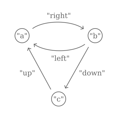
After these definitions, we're ready to follow the first example in the paper, Figure 1, which constructs a graph using edges labeled "left", "right", "up", and "down", and nodes labeled "a", "b", and "c".

([("left", 2), ("up", 3)], 1, "a", [("right", 2)]) &
([], 2, "b", [("down", 3)]) &
([], 3, "c", []) &
Empty

becomes in Python:

graph: InductiveGraph[str, str] = (
        Context(
            Adj((("left", Node(2)), ("up", Node(3)))),
            Node(1),
            "a",
            Adj((("right", Node(2)),)),
        )
        & Context(Adj(), Node(2), "b", Adj((("down", Node(3)),)))
        & Context(Adj(), Node(3), "c", Adj())
        & EmptyGraph()
)

A diagram reproducing the example in Erwig 2001, showing a directed graph with three nodes connected by four edges.

The node "a", with two predecessors and one successor, is attached to "b", with one successor, and then attached to "c", with no predecessors or successors, and finally the empty graph.

Next up

In the next article, we'll work into the next parts of the paper, which describes the properties needed from the inductive graph data types, and implement them in Python, and use them to implement some simple graph algorithms. Then, in the final section, we'll tackle some more difficult algorithms like topological sorting. Thanks for keeping up with me so far!

References

Erwig, Martin. "Inductive graphs and functional graph algorithms." Journal of Functional Programming 11.5 (2001): 467–492.

 Top