Examples
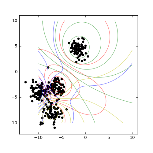
Probabilistic FCM
In the probabilistic algorithm, the total membership of every point must equal unity - that is, membership is divided between each of the possible cluster centers. Here, we produce a plot identifying the clusters in a dataset. There is overlap between the clusters where ambiguity is detected.
Input
import numpy as np
import matplotlib.pyplot as plt
from skcmeans.algorithms import Probabilistic
from sklearn.datasets import make_blobs
plt.figure(figsize=(5, 5)).add_subplot(aspect='equal')
n_clusters = 4
data, labels = make_blobs(n_samples=300, centers=n_clusters, random_state=1)
clusterer = Probabilistic(n_clusters=n_clusters, n_init=20)
clusterer.fit(data)
xx, yy = np.array(np.meshgrid(np.linspace(-10, 10, 1000), np.linspace(-10, 10, 1000)))
z = np.rollaxis(clusterer.calculate_memberships(np.c_[xx.ravel(), yy.ravel()]).reshape(*xx.shape, -1), 2, 0)
colors = 'rgbyco'
for membership, color in zip(z, colors):
    plt.contour(xx, yy, membership, colors=color, alpha=0.5)
plt.scatter(data[:, 0], data[:, 1], c='k')
Result
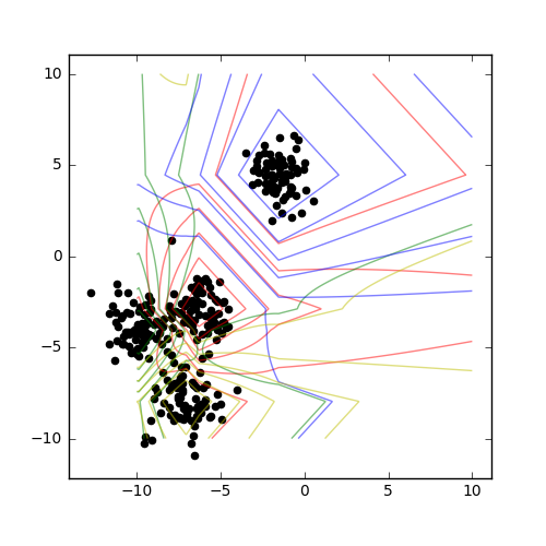
Changing the distance metric
Sometimes, it’s useful to have a look at how different distance metrics behave - for example, with higher-dimensional data, the cosine distance might do better than the default Euclidean distance. It is possible to change the distance measure of a clusterer instance on the fly, but it is probably clearer to subclass the original algorithm:
Input
import numpy as np
import matplotlib.pyplot as plt
from skcmeans.algorithms import Probabilistic
from sklearn.datasets import make_blobs
class CosineProbabilistic(Probabilistic):
    metric = 'cityblock'
plt.figure(figsize=(5, 5)).add_subplot(aspect='equal')
n_clusters = 4
data, labels = make_blobs(n_samples=300, centers=n_clusters, random_state=1)
clusterer = CosineProbabilistic(n_clusters=n_clusters, n_init=20)
clusterer.fit(data)
xx, yy = np.array(np.meshgrid(np.linspace(-10, 10, 1000), np.linspace(-10, 10, 1000)))
z = np.rollaxis(clusterer.calculate_memberships(np.c_[xx.ravel(), yy.ravel()]).reshape(*xx.shape, -1), 2, 0)
colors = 'rgbyco'
for membership, color in zip(z, colors):
    plt.contour(xx, yy, membership, colors=color, alpha=0.5)
plt.scatter(data[:, 0], data[:, 1], c='k')
Result
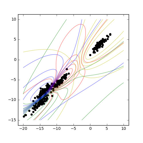
Irregular Clusters
In real data science, the clusters are not usually nice circular (or hyperspherical) shapes. One way of accounting for this is the Gustafson-Kessel algorithm, which effectively adds a covariance matrix to each cluster center, giving it ellipsoidal character, and an updated distance calculation to go with it. This can be combined with either of the basic algorithms.
Input
import numpy as np
import matplotlib.pyplot as plt
from skcmeans.algorithms import Probabilistic, GustafsonKesselMixin
from sklearn.datasets import make_blobs
class GKProbabilistic(Probabilistic, GustafsonKesselMixin):
    pass
plt.figure(figsize=(5, 5)).add_subplot(aspect='equal')
n_clusters = 4
data, labels = make_blobs(n_samples=300, centers=n_clusters, random_state=1)
transform = np.array([[1, 0.4], [1, 1]])
data = np.dot(data, transform)
clusterer = GKProbabilistic(n_clusters=n_clusters, n_init=20)
clusterer.fit(data)
xx, yy = np.array(np.meshgrid(np.linspace(-20, 10, 1000), np.linspace(-15, 10, 1000)))
z = np.rollaxis(clusterer.calculate_memberships(np.c_[xx.ravel(), yy.ravel()]).reshape(*xx.shape, -1), 2, 0)
colors = 'rgbyco'
for membership, color in zip(z, colors):
    plt.contour(xx, yy, membership, colors=color, alpha=0.5)
plt.scatter(data[:, 0], data[:, 1], c='k')
Result